Fantasy Premier League Starting Team with Linear Programming
Fantasy Premier League (FPL) : Creating the Starting Team
The Fantasy Premier League (FPL) is a popular way of engaging with the English Premier League (EPL) season, it is a competitive game where people play as managers and pick a team of EPL footballers constrained by a budget and a number of rules that determine allowed formations and limit of players from a given team. During the pre-season before the EPL restarts most premier league teams will buy and sell a number of players, so there is generally a great deal of uncertainty about who the best teams and players will be. Of course, managers (the FPL ones) are not trying to find the best players but the 11 players that will score the most points within budget.
In this notebook we assume that the points performance in the previous season, 2023/24, are the estimates of the players points in the upcoming season - naturally this is likely not the best approach, but is a good enough starting point without having to predict team and player performance - and use linear optimisation to find the optimal starting 11 and subs bench constrained by budget and the FPL rules on team formation and limits on players from each team. In FPL, managers are allowed to make one transfer each week which means that the upcoming fixtures should play a role in initial team selection because players can be transferred in and out of the team regularly.
To get the data we can use the pandas-fpl library which uses the fpl wrapper for the Fantasy Premier League API and returns the request already in a pandas dataframe.
import pandas as pd
from fplpandas import FPLPandas
import seaborn as sns
import matplotlib.pyplot as plt
import plotly.express as px
import pulp

fpl = FPLPandas()
# Fetch data using the Pandas wrapper for the FPL api:
df_players, df_players_past, df_players_history, _ = fpl.get_players()
df_teams = fpl.get_teams()
df_fixtures = fpl.get_fixtures()
# Reset index in dataframes:
df_players.reset_index(inplace=True)
df_players_past.reset_index(inplace=True)
df_players_history.reset_index(inplace=True)
df_fixtures.reset_index(inplace=True)
df_fixtures.drop(columns=['id'], inplace=True)
df_teams.reset_index(inplace=True)
# Create 23/24 players dataset and subset to players that are still in the PL this season:
df_players_recent = df_players_past[df_players_past['season_name'] == "2023/24"]
df_players_recent = df_players_recent[df_players_recent['player_id'].isin(df_players['id'])]

# Merge necessary columns from Players and Teams datasets:
df_players_recent = pd.merge(df_players_recent,
                             df_players[['id', 'first_name', 'second_name', 'element_type', 'team', 'now_cost']],
                             left_on = ['player_id'], right_on=['id'], how='left')
df_players_recent['player_name'] = df_players_recent['first_name'] + ' ' + df_players_recent['second_name']
df_players_recent.drop(columns=['id'], inplace=True)

df_players_recent = pd.merge(df_players_recent, df_teams[['id', 'name', 'strength_overall_home', 'strength_overall_away']],
                             left_on=['team'], right_on=['id'], how='left')
df_players_recent
df_players_recent.drop(columns=['id'], inplace=True)

# Create and process useful columns:
df_players_recent[['start_cost', 'end_cost', 'now_cost']] = df_players_recent[['start_cost', 'end_cost', 'now_cost']] / 10
element_type_pos_map = {1: 'GK', 2: 'DEF', 3: 'MID', 4: 'FWD'}
df_players_recent['position'] = df_players_recent.apply(lambda row: element_type_pos_map[row['element_type']], axis=1)

df_players_recent['strength_overall'] = df_players_recent[['strength_overall_home', 'strength_overall_away']].mean(axis=1)

df_players_recent['player_name'] = df_players_recent['first_name'] + ' ' + df_players_recent['second_name']
Fixture Analysis
As stated, because the FPL allows transfers through-out the season, it is beneficial to consider the opening set of fixtures for each team and potentially disallowing players from certain teams when setting up the constraints in the LP model. In this notebook we use the FPL-provided Home and Away strengths, although we could also estimate these ourselves. Teams with very difficult opening fixtures will use a lower limit on the number of players we are willing to accept from that team.
# Find teams that have the most difficult opening fixtures
df_teams['strength_overall_away'] = df_teams['strength_overall_away'] * 0.85  # adjust for home adv.
df_fixtures = pd.merge(df_fixtures, df_teams[['id', 'name', 'strength_overall_home']],
                       left_on=['team_h'], right_on=['id'])
df_fixtures.rename(columns={'name': 'home_name'}, inplace=True)
df_fixtures.drop(columns=['id'], inplace=True)

df_fixtures = pd.merge(df_fixtures, df_teams[['id', 'name', 'strength_overall_away']],
                       left_on=['team_a'], right_on=['id'])
df_fixtures.rename(columns={'name': 'away_name'}, inplace=True)
df_fixtures.drop(columns=['id'], inplace=True)

df_next_fixtures = df_fixtures[df_fixtures['event'] <= 5]  # is it int?

fixture_cols = ['team', 'opponent', 'opponent_strength']
df_next_fixtures_home = df_next_fixtures[['home_name', 'away_name', 'strength_overall_away']].copy()
df_next_fixtures_home.rename(columns={'home_name': 'team', 'away_name': 'opponent', 'strength_overall_away': 'opponent_strength'},
                             inplace=True)
df_next_fixtures_away = df_next_fixtures[['home_name', 'away_name', 'strength_overall_home']].copy()
df_next_fixtures_away.rename(columns={'away_name': 'team', 'home_name': 'opponent', 'strength_overall_home': 'opponent_strength'},
                             inplace=True)
df_next_fixture_difficulty = pd.concat([df_next_fixtures_home[fixture_cols], df_next_fixtures_away[fixture_cols]])

df_next_fixture_difficulty = df_next_fixture_difficulty.groupby(['team'])['opponent_strength'].mean().reset_index()

df_next_fixture_difficulty.sort_values(by=['opponent_strength'], ascending=False)  # ran output
We sort the table above by opponent strength, taking into account home advantage, and we decide to remove the top 6 teams except for Arsenal. We note that Arsenal have two difficult fixtures (game 4 against Man City and game 5 against Spurs) but were the clear 2nd best team last season so we do not remove their players at this stage.
remove_teams = ['Wolves', 'West Ham', 'Ipswich', 'Brentford', 'Bournemouth']
# so these teams are removed because their upcoming fixtures and on average very tough
# Note: Arsenal play Spurs and ManCity away in fixtures 4+5, we allow Arsenal players for now but might want to reconsider
Player Analysis
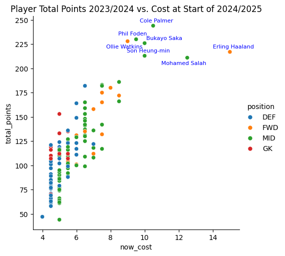
To better understand the relationship between points earned last season and the starting value this season we produce a scatter plot, highlighting the top players which are very likely to feature in the majority of FPL teams.
scatter_data = df_players_recent[df_players_recent['minutes'] > 2000]
scatter_data_subset = scatter_data[scatter_data['total_points'] > 200]
plt.figure(figsize=(8, 6))
g = sns.relplot(data=scatter_data, x="now_cost", y="total_points", hue="position")
for i in range(scatter_data_subset.shape[0]):
    if scatter_data_subset.iloc[i]['player_name'] == "Phil Foden":
        xytext_val = (-5, 6)
    elif scatter_data_subset.iloc[i]['player_name'] == "Ollie Watkins":
        xytext_val = (-5, -10)
    elif scatter_data_subset.iloc[i]['player_name'] == "Bukayo Saka":
        xytext_val = (28, 5)
    elif scatter_data_subset.iloc[i]['player_name'] == "Mohamed Salah":
        xytext_val = (-5, -10)
    else:
        xytext_val = (5, 5)
    plt.annotate(scatter_data_subset.iloc[i]['player_name'],
                 (scatter_data_subset.iloc[i]['now_cost'], scatter_data_subset.iloc[i]['total_points']),
                 textcoords="offset points", # Positioning
                 xytext=xytext_val,               # Distance from point
                 ha='center',                # Horizontal alignment
                 fontsize=8,                # Font size
                 color='blue')               # Text color
plt.title("Player Total Points 2023/2024 vs. Cost at Start of 2024/2025")
plt.show()
df_players_recent['cost_change'] = df_players_recent['now_cost'] - df_players_recent['end_cost']
scatter_data = df_players_recent[df_players_recent['minutes'] > 2000]
scatter_data_subset = scatter_data[scatter_data['total_points'] > 200]
plt.figure(figsize=(8, 6))
g = sns.relplot(data=scatter_data, x="cost_change", y="total_points", hue="position")
for i in range(scatter_data_subset.shape[0]):
if scatter_data_subset.iloc[i]['player_name'] == "Mohamed Salah":
xytext_val = (-5, -10)
elif scatter_data_subset.iloc[i]['player_name'] == "Son Heung-min":
xytext_val = (-5, 5)
elif scatter_data_subset.iloc[i]['player_name'] == "Erling Haaland":
xytext_val = (-5, -10)
elif scatter_data_subset.iloc[i]['player_name'] == "Phil Foden":
xytext_val = (-5, 8)
elif scatter_data_subset.iloc[i]['player_name'] == "Bukayo Saka":
xytext_val = (18, 5)
else:
xytext_val = (5, 5)
plt.annotate(scatter_data_subset.iloc[i]['player_name'],
(scatter_data_subset.iloc[i]['cost_change'], scatter_data_subset.iloc[i]['total_points']),
textcoords="offset points", # Positioning
xytext=xytext_val, # Distance from point
ha='center', # Horizontal alignment
fontsize=8, # Font size
color='blue') # Text color
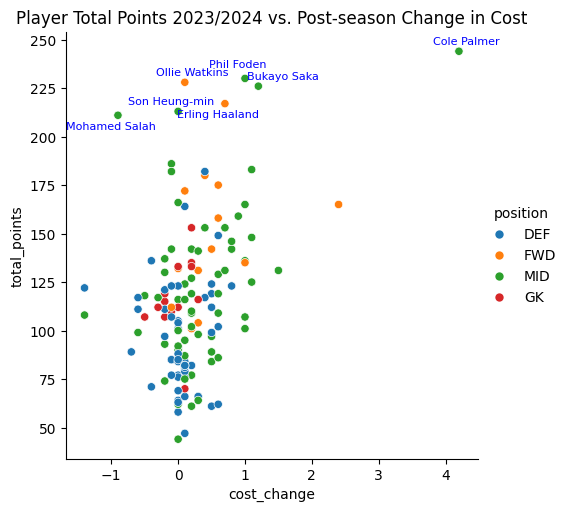
plt.title("Player Total Points 2023/2024 vs. Post-season Change in Cost")
plt.show()
Optimisation Model
The problem can be stated as optimising the total points constrained by budget, the sum of the transfer values, and the limit of players from each team and this naturally leads to a linear programming (LP) problem.
# Optimisation Model Data:
opt_data = df_players_recent[(df_players_recent['minutes'] > 2000) & ~(df_players_recent['name'].isin(remove_teams))].copy()
# You cant have spaces in names:
opt_data['player_name'] = opt_data["player_name"].apply(lambda x: ''.join([" " if ord(i) < 32 or ord(i) > 126 else i for i in x]))
opt_data['player_name'] = opt_data['player_name'].str.replace(' ', '_')
opt_data.set_index(['player_name'], inplace=True)
# Model:
lp_model = pulp.LpProblem("FPL Optimisation", pulp.LpMaximize)
player_vars = pulp.LpVariable.dicts("Player", opt_data.index, cat='Binary')
lp_model += pulp.lpSum([opt_data.loc[name, 'total_points'] * player_vars[name] for name in opt_data.index]), "Total Points"

# Budget constraint
budget = 80  # Assume we have used 20m on sub players:
# TODO change end_cost for the new season cost:
lp_model += pulp.lpSum([opt_data.loc[i, 'now_cost'] * player_vars[i] for i in opt_data.index]) <= budget, "Total Value"

# Position constraints
position_limits = {"GK": 1, "DEF": 3, "MID": 5, "FWD": 2}
for position, limit in position_limits.items():
    lp_model += pulp.lpSum([player_vars[i] for i in opt_data.index if opt_data.loc[i, 'position'] == position]) == limit, f"Exact_{position}"

# Team constraints
team_limits = {team_name: 3 for team_name in df_teams['team'] if team_name not in remove_teams}  # Example team limits
team_limits['Arsenal'] = 1  # set to 1 because of tough fixtures 4+5
team_limits['Everton'] = 1
for team, limit in team_limits.items():
    constraint = pulp.lpSum([player_vars[i] for i in opt_data.index if opt_data.loc[i, 'team'] == team])
    lp_model += constraint <= limit, f"Max_{team}"
# Run Solver:
lp_model.solve()
# Print output:
selected_players = opt_data[[player_vars[i].varValue == 1 for i in opt_data.index]]
selected_players = selected_players[['now_cost', 'total_points', 'minutes', 'team', 'position']].sort_values(by=['element_type'], ascending=True)
print("Selected players:")
print(selected_players)

# Print the total points
print("Total Points:", pulp.value(lp_model.objective))
Selected players:
                           now_cost  total_points  minutes            name  \
player_name
Jordan_Pickford                 5.0         153.0   3420.0         Everton
Benjamin_White                  6.5         182.0   2987.0         Arsenal
Joachim_Andersen                4.5         121.0   3416.0  Crystal Palace
Pedro_Porro                     5.5         136.0   3090.0           Spurs
Pascal_Gro_                     6.5         153.0   3112.0        Brighton
Cole_Palmer                    10.5         244.0   2617.0         Chelsea
Phil_Foden                      9.5         230.0   2860.0        Man City
Rodrigo_'Rodri'_Hernandez       6.5         159.0   2931.0        Man City
Anthony_Gordon                  7.5         183.0   2896.0       Newcastle
Ollie_Watkins                   9.0         228.0   3222.0     Aston Villa
Alexander_Isak                  8.5         172.0   2253.0       Newcastle

                          position  element_type
player_name
Jordan_Pickford                 GK             1
Benjamin_White                 DEF             2
Joachim_Andersen               DEF             2
Pedro_Porro                    DEF             2
Pascal_Gro_                    MID             3
Cole_Palmer                    MID             3
Phil_Foden                     MID             3
Rodrigo_'Rodri'_Hernandez      MID             3
Anthony_Gordon                 MID             3
Ollie_Watkins                  FWD             4
Alexander_Isak                 FWD             4
Total Points: 1961.0
We ran the LP algorithm multiple times, one for each possible formation allowed in the FPL rules.
# 442:
print(f"442 - cost:{selected_players[['now_cost']].sum().iloc[0]} and points:{selected_players[['total_points']].sum().iloc[0]}")
442 - cost:80.0 and points:2001.0
# 352:
print(f"352 - cost:{selected_players[['now_cost']].sum().iloc[0]} and points:{selected_players[['total_points']].sum().iloc[0]}")
352 - cost:80.0 and points:2009.0
# 433:
print(f"433 - cost:{selected_players[['now_cost']].sum().iloc[0]} and points:{selected_players[['total_points']].sum().iloc[0]}")
433 - cost:80.0 and points:1992.0
Substitutes
We repeat the LP algorithm to find the substitute bench; we adjust the player team limits for the starting 11 we found above.
opt_substitute_data = opt_data[~opt_data.index.isin(selected_players.index)]

# Model:
lp_model = pulp.LpProblem("FPL Optimisation", pulp.LpMaximize)
player_vars = pulp.LpVariable.dicts("Player", opt_substitute_data.index, cat='Binary')
lp_model += pulp.lpSum([opt_substitute_data.loc[name, 'total_points'] * player_vars[name] for name in opt_substitute_data.index]), "Total Points"

# Budget constraint
budget = 20  # Assume we have used 20m on sub players:
# TODO change end_cost for the new season cost:
lp_model += pulp.lpSum([opt_substitute_data.loc[i, 'now_cost'] * player_vars[i] for i in opt_substitute_data.index]) <= budget, "Total Value"

# Position constraints
position_limits = {"GK": 1, "DEF": 2, "MID": 0, "FWD": 1}
for position, limit in position_limits.items():
    lp_model += pulp.lpSum([player_vars[i] for i in opt_substitute_data.index if opt_substitute_data.loc[i, 'position'] == position]) == limit, f"Exact_{position}"

# Team constraints
team_limits = {team_name: 3 for team_name in df_teams['name'] if team_name not in remove_teams}  # Example team limits
team_limits['Newcastle'] = 1  # set to 1 because of tough fixtures 4+5
team_limits['Man City'] = 1
team_limits['Everton'] = 0
team_limits['Fulham'] = 1
for team, limit in team_limits.items():
    constraint = pulp.lpSum([player_vars[i] for i in opt_substitute_data.index if opt_substitute_data.loc[i, 'name'] == team])
    lp_model += constraint <= limit, f"Max_{team}"
    # lp_model += pulp.lpSum([player_vars[i] for i in opt_data.index if opt_data.loc[i, 'team'] == team]) <= limit, f"Max_{team}"
# Run Solver:
lp_model.solve()
# Print output:
selected_players_sub = opt_substitute_data[[player_vars[i].varValue == 1 for i in opt_substitute_data.index]]
selected_players_sub = selected_players_sub[['now_cost', 'total_points', 'minutes', 'name', 'position']].sort_values(by=['element_type'], ascending=True)
print("Selected players:")
print(selected_players_sub)

# Print the total points
print("Total Points:", pulp.value(lp_model.objective))
Selected players:
                               now_cost  total_points  minutes  \
player_name
Andr__Onana                         5.0         133.0   3420.0
Tyrick_Mitchell                     5.0         119.0   3204.0
Timothy_Castagne                    4.5         105.0   2630.0
Jo_o_Pedro_Junqueira_de_Jesus       5.5         104.0   2037.0

                                         name position  element_type
player_name
Andr__Onana                           Man Utd       GK             1
Tyrick_Mitchell                Crystal Palace      DEF             2
Timothy_Castagne                       Fulham      DEF             2
Jo_o_Pedro_Junqueira_de_Jesus        Brighton      FWD             4
Total Points: 461.0